
A/B Testing
1. Overview
1.1 What is A/B Testing?
A general methodology used online when you wanna test out a new product or a feature. Use two sets of users: control set (existing product) and experiment set (new version) by obsevering how these users respond differently to determine which version of feature/product is better.
1.2 Pros & Cons
- useful: 1) help you climb to the peak of your current mountain
- not useful:
- test new experiences; old users may resist against the new version (change aversion), or old users may all go for the new experience, then test everything (novelty effect). Two issues to consider when it comes to a new experience: (1) what is your baseline of comparison? (2) how much time do you need in order for your users to adapt to the new experience, so that you can actually say what is the plateaued experience and make a robust decision?
- long term effect is hard to test too, such as a website that recommends apartment rentals; note update brand or logo can’t use ab testing, it’s surprisingly emotional and users need some time to get used to new logo
- can’t really tell you if you’re missing something
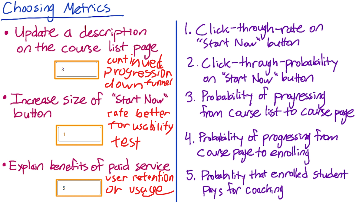
1.3 Choose a metric
\[click\ through\ rate = \frac{number\ of\ clicks}{number\ of\ page\ views}\] \[click\ through\ probability = \frac{unique\ vistors\ who\ clicks}{unique\ vistors\ to\ page}\]Binomial Distribution
- 2 Types of outcomes (success/failure)
- The probability of success (p) stays the same from one trial to another. The probability of failure (q) = 1 – p
- All trials are independent
- Identical distribution (i.e p same for all)
One sample Z test about p
- Assumption:
- population is large enough to invoke the CLT (To use normal): N > 25, $N\ *\ \hat{p}$ > 5 and $N\ (1- \hat{p})$ > 5
- Expection probability: $\hat{p} = \frac{X}{N}$
- Standard deviation: $\sqrt{\frac{\hat{p}(1-\hat{p})}{N}}$
- margin of error = $Z \ *\ \sqrt{\frac{\hat{p}(1-\hat{p})}{N}}$
- Z = $\frac{\hat{p}\ -\ p}{\sqrt{\frac{\hat{p}(1-\hat{p})}{N}}}$
- $\hat{d}$ = $\frac{X_{exp}}{N_{exp}}\ -\ \frac{X_{control}}{N_{control}} $
-
Confidence interval = $\hat{p}$ +- ME (margin of error)
- Practical significant: refers to the real-world importance or meaningfulness of an effect or result.
- 比如通过考试成绩来判断study program的有效性,我们把5%认定为是有practical significant (i.e. an efffect of 4 points or less is too small to care about). 在进行了实验后,我们发现两组有statistically significant difference,参加study program的人得分比没参加的多了3%(百分制)。然而根据先前定的practical significant 来看,3%是小于5%的,所以即使我们的实验证明了study program确实能提高分数,但在现实情况下,参与者在study program上所花的时间和金钱不值得只提高3%。
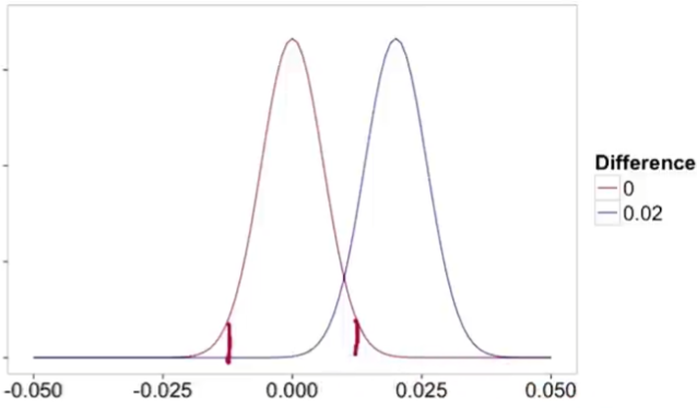
Size V.S. power trade-off
Statistical power helps us find how many samples do we need to have statistical significance.
$\alpha$ = P(reject null I null TRUE) 拒绝了原本对的,误报 (false positive)
$\beta$ = P(fail to reject I null FALSE) 接受了本该错的,漏报 (false negative)
sensitivity = 1 - $\beta$, often 80%
Small sample: $\alpha$ low, $\beta$ high
Large sample: $\alpha$ same, $\beta$ low
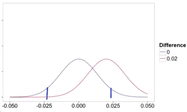
confidence interval case breakdown
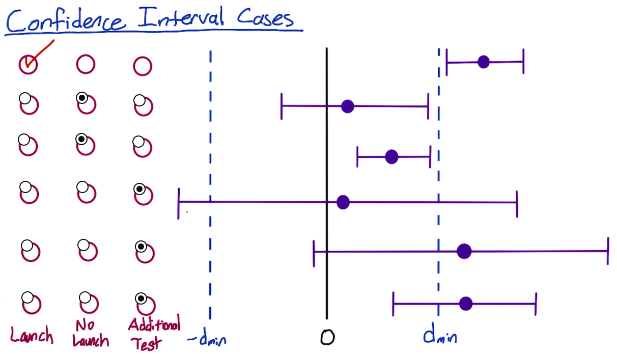
- case2: neutral change
- case4: the confidence interval bounds are outside of what’s practically significant, it could be causing them to increase or decrease
- case5: confidence interval overlaps 0, there might not even be a change at all
- case6: it’s possible your change is not practically significant
2. Choosing and Characterizing Metrics
Types of Metrics:
- Sanity checking metrics (Invariant Metrics) — can be multiple metrics. Eg. When changing the page and testing CTR, latency & load times should be invariant
- Evaluation metrics — one or multiple.
For multiple metrics, composite metrics and OEC (overall evaluation criterion), they are hard to define (it need to agree on a definition/end up looking all the individual metrics).
Metric Definition
- come up with a high-level concept for a metric, such as “active users”, which can be understood by everyone.
- details: how do you define “active”;
- summarize all of these individual data measurements into a single metric such as count or sum;
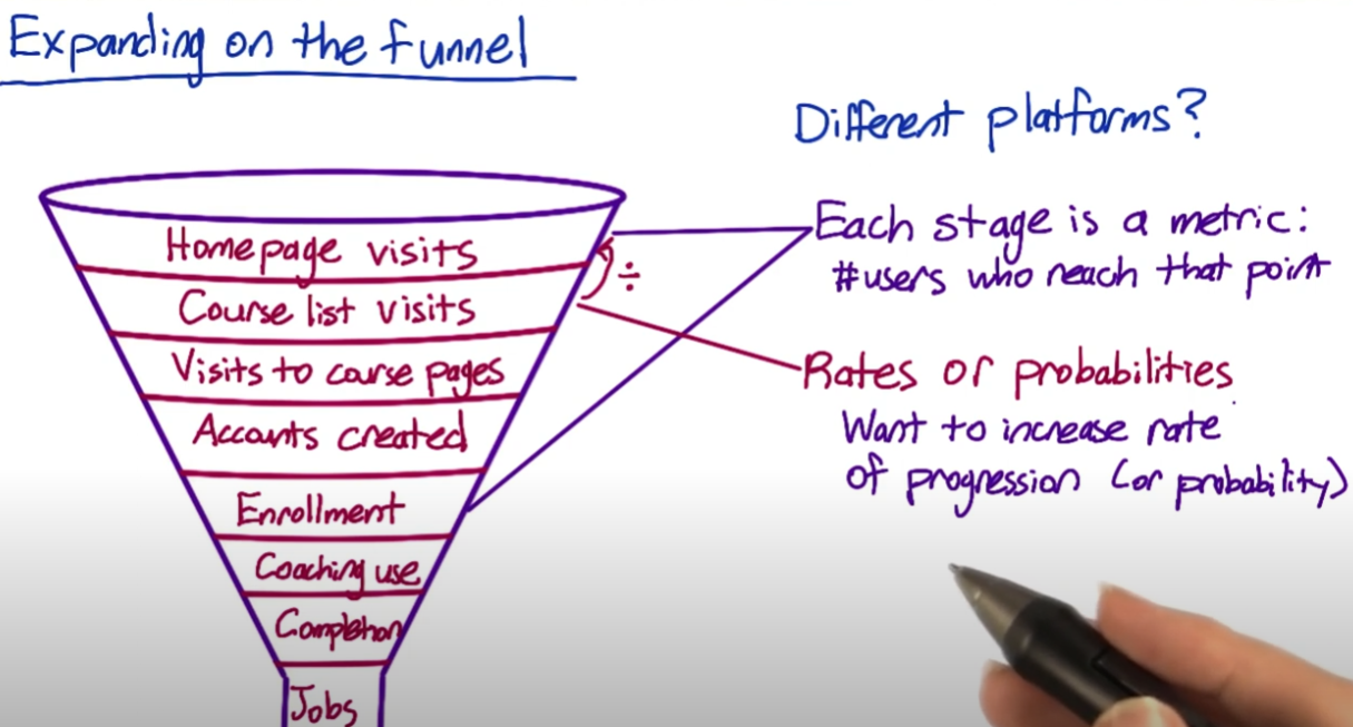
Refining the customer funnel (Udacity example)
- Homepage visits
- Exploring the site
- Users who view course list
- Users who view course details
- Create an account
- Users who enroll in a course
- Users who finish lesson 1,2,etc.
- Users who sign up for coaching at various levels
- Completing a course
- Users who enroll in a second class
- Users who gets jobs
Metric Choosing
Difficult metrics
- Don’t have access to data
- takes too long
Technique to deal with difficulty
- External Data: Use industry metrics from external data (Neilson, comscore), Survey data (Pew, Forrester), Academic research.
- Internal Existing Data: Retrospective analysis (correlation but not causation), running experiments, user experience research, surveys, and focus groups.
Retrospective analysis: used to look at how a metric changes in response to past changes or experiments. This can help establish a baseline and develop theories.
Techniques to Gather Additional Data
-
User Experience Research (UER)
+good for brainstorming
+can use special equipment (catch eye movement)
-want to validate results
-
Focus Groups
+get feedback on hypotheticals
-Run the risk of group think
-
Surveys
+Useful for metrics you cannot directly measure (whether student who take course get job)
-Can’t directly compare to other results (more observational methods)
Metric definitions
High-level metric: click through probability: $\frac{users\ who\ click}{users\ who\ visit}$
-
Def #1 (Cookie probability): For each time interval, $\frac{number\ of\ cookies\ that\ click} {number\ of\ cookies}$, for users who clicks the back button and returns to a previously visited page, the browser may retrieve the cached version of that page instead of making a new request to the server. 即返回前一页, present cookie仍存在。
-
Def #2 (Pageview probability): $\frac{Number\ of\ pageviews\ with\ a\ click\ within\ time\ interval}{number\ of\ pageviews}$
-
Def #3 (Rate): $\frac{Number\ of\ clicks}{Number\ of\ pageviews}$
Summary Metrics
Establish a few characteristics for your metric:
- Sensitivity and robustness
- Characterize the distribution: retrospective analysis
Four categories of metrics to keep in mind:
- sums and counts
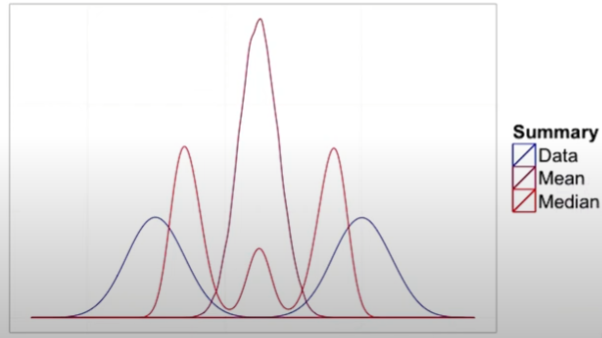
- Distributional metrics: means, median, and percentiles (75th, 90th)
- Probabilities and rates
- Ratios
Sensitivity: how well a metric can detect changes that you care about
Robustness: the metric’s ability to remain stable when there are changes that you don’t care about, it doesn’t move a lot when nothing interesting has happened.
2 WAYS to Measure:
- Running experiments, a/a experiment to determine if they’re too sensitive.
- Retrospective analysis of your logs (robustness). Involving looking back at past experiments or changes made to the website and examining if the metric values moved in conjunction with those changes (if remain stable or show minimal change, indicate robust).
- Analyze the history of the metric and try to find causes for any major changes observed (hindsight). It can provide valuable insight into the behavior of the metric over time and help you understand its robustness.
Absolute vs. relative difference
Suppose you run an experiment where you measure the number of visits to your homepage, and you measure 5000 visits in the control and 7000 in the experiment. Then the absolute difference is the result of subtracting one from the other, that is, 2000. The relative difference is the absolute difference divided by the control metric, that is, 40% ($\frac{2000}{5000} * 100\%$).
Variability
| Type of Metric | Distribution | Estimated Variance |
|---|---|---|
| Probability | binomial (normal) | $\sqrt{\frac{\hat{p}(1-\hat{p})}{N}}$ |
| mean | normal | $\frac{\sigma^2}{N}$ |
| median/percentile | depends 1 | depends |
| count/difference | normal (maybe) | Var(X) + Var(Y) |
| rates | poisson2 | $\bar{X}$ |
| ratios | depends3 | depends |
-
median - could be non-normal if data is non-normal
-
extreme version of normal distribution, N super large, p super small. 泊松分布是指某段连续的时间内某件事情发生的次数,而且“某件事情”发生所用的时间是可以忽略的。例如,在五分钟内,电子元件遭受脉冲的次数,就服从于泊松分布。假如你把“连续的时间”分割成无数小份,那么每个小份之间都是相互独立的。在每个很小的时间区间内,电子元件都有可能“遭受到脉冲”或者“没有遭受到脉冲”,这就可以被认为是一个p很小的二项分布。而因为“连续的时间”被分割成无穷多份,因此n(试验次数)很大。所以,泊松分布可以认为是二项分布的一种极限形式。
-
different ratio use different data, so it depend on the distribution for the numerator and the denominator of the ratio.
Empirical Variability
- For complicated metrics, the distribution can be weird. You might want to shift to an empirical estimate.
- A/A testing: control A against another control A, and there’s actually no change in what the users are seeing. What that means is that any differences that you measure are due to the underlying variability, maybe of your system or the user population, what users are doing, all of those types of things.
- Pros: If your experiment system is itself complicated, it’s actually a good test of your system.
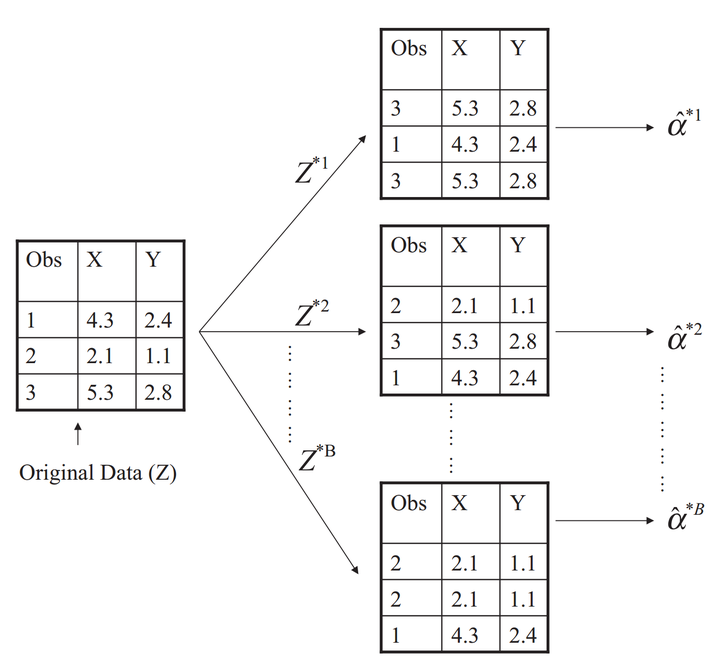
- Bootstrap: 将一个大样本按照有放回的取样方法,取出一定数量的新样本,把这些random subset当作simulated experiment. In reality, what we have is a whole gradation of different methods. If the bootstrap estimate is agreeing with your analytical estimate, you can probably move on. If not, consider big A/A testing.
Uses of A/A Test
- Compare results to what you expect (sanity check). Example
- Estimate variance and calculate confidence
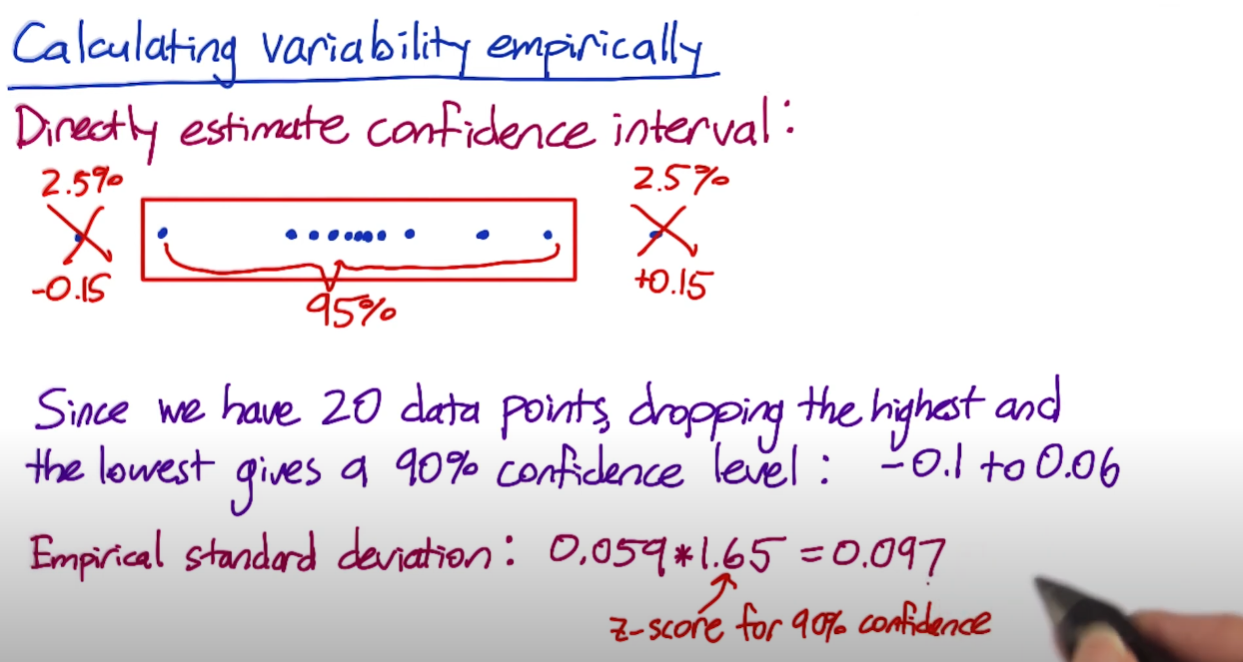
- Directly estimate confidence interval
3. Design an experiment
Unit of Diversion Overview
A unit of diversion is how we define what an individual subject is in the experiment. 根据unit of diversion去分配individual到不同的组中. 见下面的example。
You are doing an event based diversion, a cookie-based, or a user id, these are all what we call our unit of diversion.
Commonly used
- User id
- stable, unchanging
- personally identifiable
- Anonymous id (cookie)
- change when switch device (laptop to mobile) OR browser (chrome to safari)
- users can clear cookie
- Event
- no consistent experience
- use only for non-user-visible changes
Less Common
- Device id
- only available for mobile
- tied to specific device
- unchangeable by user
- personally identifiable
- IP address
- change when location changes
Three main Considerations when choosing diversion
- User consistency
- Most users will not notice ranking changes, so event-based diversion is good
- event < cookie < id
- Ethical consideration for diversion
- Variability
Unit of analysis: the denominator of the metric
- when your unit of analysis = unit of diversion, then the variability tends to be lower and close to the analytical estimate.
Inter- vs. Intra-user Experiments
- Intra-user Experiment: expose the same user to the feature being on/off over time.
- Interleaved Experiment: expose the same user to the A and the B side at the same time. Typically, this only work in cases where you are looking at reordering a list.
- Inter-user experiment: got different ppl on the A side and on the B side. i.e. AB testing
population vs. cohort
Cohort: a group of individuals who share a common characteristic or experience, also a subset of population.
Use cohort instead of population when you are looking for learning effects, examining user retention, want to increase user activity, or anything requiring user to be established.
Sizing
The size of the experiment is determined based on practical significance, statistical significance, and the desired sensitivity. (example)
It is also important to consider factors such as the choice of metric, unit of diversion, significant level ($\alpha$), reduced power (1 - $\beta$) (i.e. increase $\beta$) and population, as these can affect the variability of the metric.
Taken Udacity as example, there are three possible way to reduce the size of an experiment
- Change unit of diversion to page view
- Makes unit of diversion same as unit of analysis
- Target experiment to specific traffic
- non-English traffic will dilute the results
- could impact choice of practical significance boundary
- Change metric to cookie-based click through probability
- often doesn’t make significant difference
- If there is a difference, variability would probably go down
Duration vs. Exposure
What fraction of your traffic you’re going to send through the experiment? The duration of your experiment is related to the proportion of traffic you’re sending through your experiment.
We couldn’t run on all of traffic to get results quicker for several reasons:
- safety to make sure the function works well;
- press we don’t want a lot of people to know it before it works;
- other things impact the variability such as holiday.
Learning Effect
-
When there’s a new change in the beginning, users may against the change (change version) or use the change a lot (novelty effect). But over time, user behavior becomes stable, which is called the plateau stage. The key thing to measure learning effect is time, but in reality, you don’t have that much luxury of taking that much time to make a decision. Suggestion: run on a smaller group of users for a longer period of time.
- If you do have much time, you also need to notice the following points:
- choosing the unit of diversion correctly;
- dosage: how often we see the change, then you probably want to be using cohort as opposed to just a population;
- risk and duration.
- Pre-periods and post-periods: A/A test before and after the experiment.
4. Analyzing Results
Sanity Check
- Choosing invariant metrics (1. population sizing metrics 2. other metrics don’t expect to change)
- checking invariants
Example: experiment for two weeks
Total control: 64454 Total experiment: 61818
Whether the difference is within expectations?
Solution 1:
-
Compute standard deviation of binomial with probability 0.5 of success (coin situation)
SD = $\sqrt{\frac{0.5 * 0.5}{64454\ +\ 61818}}$ = 0.0014
-
Multiply by z-score to get margin of error
m = SD * 1.96 (95% confidence interval) = 0.0027
-
Compute confidence interval around 0.5
0.4973 (0.5 - 0.0027) to 0.5027 (0.5 + 0.0027)
-
Check whether observed fraction is within interval
$\hat{p}$ = $\frac{64454}{64454\ +\ 61818}$ = 0.5104 > 0.5027, so sth is incorrect.
Solution 2:
Checking whether any particular day (weekend, holiday) stands out as causing the problem or whether it seems to be an overall pattern.
Signal Metric
Effect Size
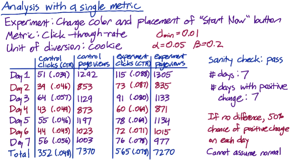
The effect size test is statistically significant if the confidence interval does not include zero, and the sign test is statistically significant if the p-value < alpha (retain H0).
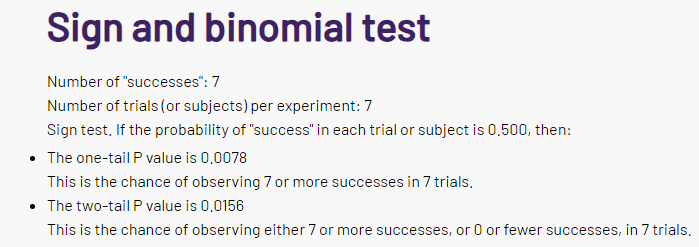
Sign Test (non-parameter)
The two-tail p value is 0.0156 < 0.05, reject H0,meaning there is difference between the control and experimental groups.
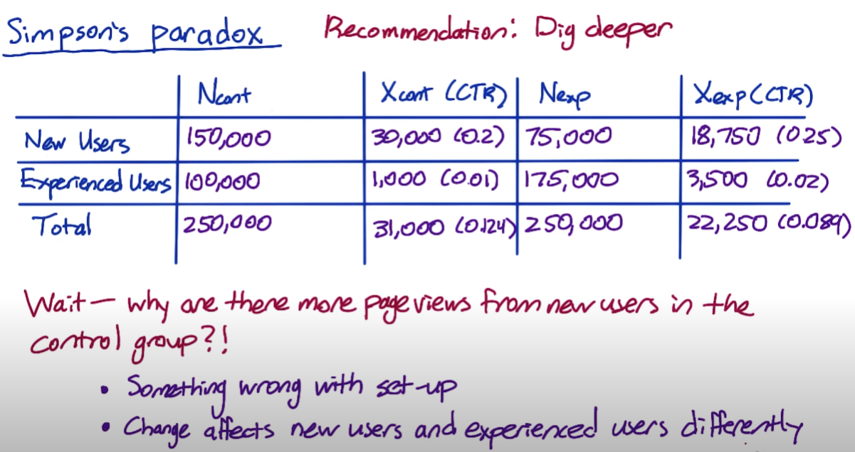
Simpson’s Paradox
Simpson’s Paradox is a phenomenon in statistics where within each subgroup, the results are stable. However, when you aggregate them all together, it’s the mix of subgroups that actually drives your result. 类似极值影响overall,需要判断是否change争对不同的group (control/experiment)。
Multiple metrics
As you test more metrics, it becomes more likely that one of them will show a statistically significant result by chance.
For example, let’s say there are 3 metrics, what’s the chance of at least 1 false positive? Assuming metrics are independent.
P(FP = 0) = 0.95 * 0.95 * 0.95 = 0.857
P(FP >= 1) = 1 - 0.857 = 0.143
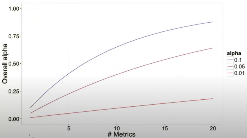
Problem: probability of any FP increases as increase number of metrics.
Solution: Use higher confidence level for each metric
Method 1: Assume independence
- $\alpha$overall = 1 - (1 - $\alpha$individual) N
Method 2: Bonferroni Correction
- no assumption
- conservative: guaranteed to give $\alpha$overall at least as small as specified
Other Method
-
Familywise error rate (FWER): control probability that any metrics shows a FP, AKA $\alpha$overall
-
False discovery rate (FDR): across a large number of metrics
FDR = E[$\frac{false\ positives}{rejections}$]
suppose there are 200 metrics, cap FDR at 0.05. This means u’r okay with 5 FP and 95 true positives in every experiment.
Drawing Conclusions:
- Do I have statistically significant and practically significant results in order to justify the change?
- Do I understand what that change has actually done with regards to user experience?
- Is it worth it?
Gotchas: Changes over time.
When you are ramping up the change, you may see the effect flatten out, thus making the tested effect not repeatable. There are many reasons for this phenomenon:
- Seasonality effect, event-driven impact; Solution: Use hold-back method. Launch the change to everyone except for one small hold-back group of users and continue comparing their behavior to the control group.
- Novelty effect or change aversion: Cohort analysis may be helpful.